HOME | DD
 FractalMonster — CubicBudCompass
by-nc-sa
FractalMonster — CubicBudCompass
by-nc-sa

Published: 2009-11-03 22:07:02 +0000 UTC; Views: 384; Favourites: 16; Downloads: 21
Redirect to original
Description
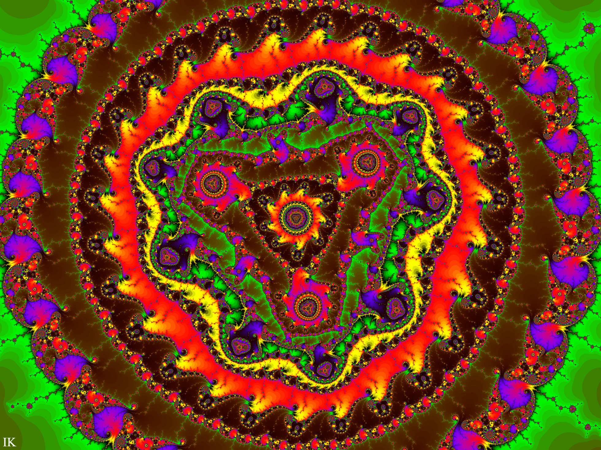
Download for 1280x960 resolutionThis is my very first published fractal motive from heptic parameter space [link] (see the linked journal).
*a_real = #pixel (horizontal)
*a_imag = #pixel (vertical)
*b_real = 0.5
*b_imag = 0
*c_real = -0.5
*c_imag = 0
*d_real = -0.5
*d_imag = 0
*e_real = 0.5
*e_imag = 0
*f_real = 0
*f_imag = 0
The black area in the middle is (a 2D slice) of Heptic Connectedness Locus (HCL), the set for which ALL the six critical points has bounded orbits. The fractal border of HCL is formed of M1 and M6 that completely coalesce in this slice. The borders of M2, M3, M4, and M5 also completely coalesce in this slice and form all the outer fractal borders (including the islands).
This motive came up as one of the big surprises from the heptic (7th) degree) parameter space. It’s like the cubic compass [link] (see also figure 1 in [link] ), which also occurs in pentic parameter space, see [link] , and as we shall see later here in Heptics also. But here the buds of the outer circle are Cubic Mandelbrot buds having (of cause) Cubic minibrots in their filaments. The islands that surrounds the compass is also made up of cubic mandys (we will see that later).
Note: This motive is a one layer image drawn due to HCL + SetBorders visualizing all the sets in one layer.
Instead of the basic coloring (coloring according to the number of iterations) a evaluated form called Continius Potential Method (CPM) is used. This method produces continues slopes around the sets instead of discrete plateaus.
No filters or post processing.
Below the UF parameter file. Play and have fun
 (Smile)")
CubicBudCompass {
fractal:
title="CubicBudCompass" width=640 height=480 layers=1
credits="Ingvar Kullberg;11/3/2009"
layer:
caption="HCL+SetBorders" opacity=100 method=multipass
mapping:
center=0/0 magn=0.53432614
formula:
maxiter=500 filename="sp3.ufm" entry="HepticParameterspace3"
p_PlottedPlane="1.(a-real,a-imag)" p_M=HCL p_SetBorders=yes
p_hide=yes p_areal=0.0 p_aimag=0.0 p_breal=0.5 p_bimag=0.0
p_creal=-0.5 p_cimag=0.0 p_dreal=-0.5 p_dimag=0.0 p_ereal=0.5
p_eimag=0.0 p_freal=0.0 p_fimag=0.0 p_xrot=0.0 p_yrot=0.0
p_xrott=0.0 p_yrott=0.0 p_xrotu=0.0 p_yrotu=0.0 p_xrotv=0.0
p_yrotv=0.0 p_xrotr=0.0 p_yrotr=0.0 p_xrots=0.0 p_yrots=0.0
p_xrota=0.0 p_yrota=0.0 p_xrotb=0.0 p_yrotb=0.0 p_xrotc=0.0
p_yrotc=0.0 p_xrotd=0.0 p_yrotd=0.0 p_zrot=0.0 p_LocalRot=no
p_diff=no p_bailout=100.0 p_dbailout=1E-6
inside:
transfer=none
outside:
density=0.1 transfer=linear filename="spr.ucl"
entry="ContinousPotential" p_auto=yes p_auton=10.0 p_n=1.0
p_numfact=1.0 p_scale=1.0 p_smooth=no p_epsilon=0.5 p_illustr=no
p_limiton=no p_limit=0.1 p_index3=0.0 p_index1=0.99 p_index2=0.0
p_speed=0.5 p_acc=1.0 p_clog=yes p_power=2.0 p_reversed=no p_test=no
p_testvalue=0.7 p_index4=0.29
gradient:
smooth=yes rotation=-77 index=20 color=16777215 index=105
color=1776680 index=192 color=7235583 index=-100 color=1709594
index=-72 color=16777215 index=-7 color=2827308
opacity:
smooth=no index=0 opacity=255
}